Probabilistic Data Structures for Web Analytics and Data Mining

Let us start with a simple example that illustrates capabilities of probabilistic data structures:

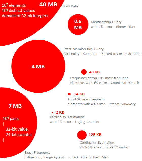
原始数据是10m个32位整数，但是去重之后个数只有1m个，占用40MB存储空间。在这个原始数据上做下面这些查询：

• How many distinct elements are in the data set (i.e. what is the cardinality of the data set)? （去重元素个数）
• What are the most frequent elements (the terms “heavy hitters” and “top-k elements” are also used)?（频率TopK 查询）
• What are the frequencies of the most frequent elements?（具体频率查询）
• How many elements belong to the specified range (range query, in SQL it looks like SELECT count(v) WHERE v >= c1 AND v < c2)?（符合范围元素个数查询）
• Does the data set contain a particular element (membership query)?（存在性查询）

The picture above shows (in scale) how much memory different representations of the data set will consume and which queries they support:（可以看到，这些概率性数据结构，通常假设数据集合是skewed的。这样对于高频和低频都保持在比较低的错误率上）

• A straightforward approach for cardinality computation and membership query processing is to maintain a sorted list of IDs or a hash table. This approach requires at least 4MB because we expect up to 10^6 values, the actual size of the hash table will be even larger.
• A straightforward approach for frequency counting and range query processing is to store a map like (value -> counter) for each element. It requires a table of 7MB that stores values and counters (24-bit counters are sufficient because we have not more than 10^7 occurrences of each element).
• With probabilistic data structures, a membership query can be processed with 4% error rate (false positive answers) using only 0.6MB of memory if data is stored in the Bloom filter.（Bloom filter来做存在性查询）
• Frequencies of 100 most frequent elements can be estimated with 4% precision using Count-Min Sketch structure that uses about 48KB (12k integer counters, based on the experimental result), assuming that data is skewed in accordance with Zipfian distribution that models well natural texts, many types of web events and network traffic. A group of several such sketches can be used to process range query.（Count-Min Sketch方法对于skewed dataset非常有效）
• 100 most frequent items can be detected with 4% error (96 of 100 are determined correctly, based on the experimental results) using Stream-Summary structure, also assuming Zipfian distribution of probabilities of the items.（Stream-Summary同样假设skewed dataset）
• Cardinality of this data set can be estimated with 4% precision using either Linear Counter or Loglog Counter. The former one uses about 125KB of memory and its size is linear function of the cardinality, the later one requires only 2KB and its size is almost constant for any input. It is possible to combine several linear counters to estimate cardinality of the corresponding union of sets.（HyperLogLog来做去重次数统计）

A number of probabilistic data structures is described in detail in the following sections, although without excessive theoretical explanations – detailed mathematical analysis of these structures can be found in the original articles. The preliminary remarks are: For some structures like Loglog Counter or Bloom filter, there exist simple and practical formulas that allow one to determine parameters of the structure on the basis of expected data volume and required error probability. Other structures like Count-Min Sketch or Stream-Summary have complex dependency on statistical properties of data and experiments are the only reasonable way to understand their applicability to real use cases.（对于LogLog Counter和Bloom Filter存在数学上的证明来决定参数以达到某种误差概率，而其他的数据结构比如Count-Min Sketch或者是Stream-Summary参数上的选择则完全依赖于统计数据，所以只能够通过实验来分析）

这个算法比较简单。首先维护一个全0的bitset, 之后对每个value做hash，映射到bitset对应的bit并且置1。处理完所有的value之后统计这个bitset有多少个bit置1，这个数目就是cardinality.

Let’s say that the ratio of a number of distinct items in the data set to m is a load factor. It is intuitively clear that: (load factor = number of distinct items / m)

• If the load factor is much less than 1, a number of collisions in the mask will be low and weight of the mask (a number of 1’s) will be a good estimation of the cardinality.
• If the load factor is higher than 1, but not very high, many different values will be mapped to the same bits. Hence the weight of the mask is not a good estimation of the cardinality. Nevertheless, it is possible that there exist a function that allows one to estimate the cardinality on the basis of weight (real cardinality will always be greater than weight).
• If the load factor is very high (for example, 100), it is very probable that all bits will be set to 1 and it will be impossible to obtain a reasonable estimation of the cardinality on the basis of the mask.

The following table contains key formulas that allow one to estimate cardinality as a function of the mask weight and choose parameter m by required bias or standard error of the estimation:

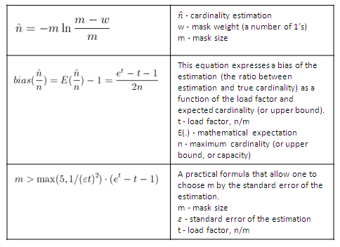
The rule of thumb is that load factor of 10 can be used for large data sets even if very precise estimation is required, i.e. memory consumption is about 0.1 bits per unique value. This is more than two orders of magnitude more efficient than the explicit indexing of 32- or 64-bit identifiers, but memory consumption grows linearly as a function of the expected cardinality (n), i.e. capacity of counter.（load factor在10左右可以获得比较高的精度，在加上1 byte = 8 bits, 空间大小可以节省大约两个数量级）

这个算法 之前(HyperLogLog这节) 分析过

The following table provides the estimation formula and equations that can be used to determine numerical parameters of the Loglog Counter:

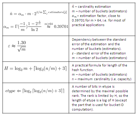
These formulas are very impressive. One can see that a number of buckets is relatively small for most of the practically interesting values of the standard error of the estimation. For example, 1024 estimators provide a standard error of 4%. At the same time, the length of the estimator is a very slow growing function of the capacity, 5-bit buckets are enough for cardinalities up to 10^11, 8-bit buckets (etype is byte) can support practically unlimited cardinalities. This means that less than 1KB of auxiliary memory may be enough to process gigabytes of data in the real life applications! （bucket数量的增长相对与原始数据量的增长是非常缓慢的）

The basic idea of Count-Min Sketch is quite simple and somehow similar to Linear Counting. Count-Min sketch is simply a two-dimensional array (d x w) of integer counters. When a value arrives, it is mapped to one position at each of d rows using d different and preferably independent hash functions. Counters on each position are incremented. This process is shown in the figure below:

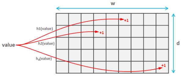
It is clear that if sketch is large in comparison with the cardinality of the data set, almost each value will get an independent counter and estimation will precise. Nevertheless, this case is absolutely impractical – it is much better to simply maintain a dedicated counter for each value by using plain array or hash table. To cope with this issue, Count-Min algorithm estimates frequency of the given value as a minimum of the corresponding counters in each row because the estimation error is always positive (each occurrence of a value always increases its counters, but collisions can cause additional increments). A practical implementation of Count-Min sketch is provided in the following code snippet.

一个value会映射到每个row上面某个column。因为对于某一个cell来说可能会有不同的value重复叠加这个单元。如果sketch比较大的，那么对应某个row来说其中的column被重复叠加的概率就比较小，而这个column的值肯定是比其他row上面对应的column要小的。

class CountMinSketch {
    long estimators[][] = new long[d][w]    // d and w are design parameters
    long a[] = new long[d]
    long b[] = new long[d]
    long p      // hashing parameter, a prime number. For example 2^31-1
    void initializeHashes() {
        for(i = 0; i < d; i++) {
            a[i] = random(p)    // random in range 1..p
            b[i] = random(p)
        }
    }
    void add(value) {
        for(i = 0; i < d; i++)
            estimators[i][ hash(value, i) ]++
    }
    long estimateFrequency(value) {
        long minimum = MAX_VALUE
        for(i = 0; i < d; i++)
            minimum = min(
                minimum,
                estimators[i][ hash(value, i) ]
            )
        return minimum
    }
    hash(value, i) {
        return ((a[i] * value + b[i]) mod p) mod w
    }
}

Dependency between the sketch size and accuracy is shown in the table below. It is worth noting that width of the sketch limits the magnitude of the error and height (also called depth) controls the probability that estimation breaks through this limit:

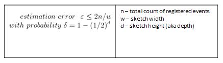
count-min sketch这种算法只有在dataset本身比较skewed的情况下才能够获得比较好的结果，也就是说如果d x w比较小的话，那么对于skewed dataset是比较合适的。

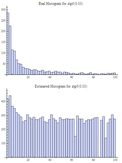
Two experiments were done with the Count-Min sketch of size 3×64, i.e. 192 counters total. In the first case the sketch was populated with moderately skewed data set of 10k elements, about 8500 distinct values (element frequencies follow Zipfian distribution which models, for example, distribution of words in natural texts). The real histogram (for most frequent elements, it has a long flat tail in the right that was truncated in this figure) and the histogram recovered from the sketch are shown in the figure below:

In the second case the sketch was populated with a relatively highly skewed data set of 80k elements, also about 8500 distinct values. The real and estimated histograms are presented in the figure below:

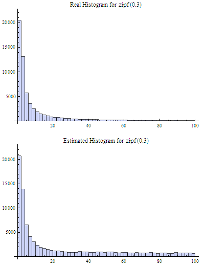
One can see that result is more accurate, at least for the most frequent items. In general, applicability of Count-Min sketches is not a straightforward question and the best thing that can be recommended is experimental evaluation of each particular case.

对于low or moderately skewed dataset来说，hash冲突比较严重所以会导致结果偏差比较大。我们可以通过去除相互影响的噪音来解决这个问题。

As an alternative, more careful correction can be done to compensate the noise caused by collisions. One possible correction algorithm was suggested in (5). It estimates noise for each hash function as the average value of all counters in the row that correspond to this function (except counter that corresponds to the query itself), deduces it from the estimation for this hash function, and, finally, computes the median of the estimations for all hash functions. Having that the sum of all counters in the sketch row equals to the total number of the added elements, we obtain the following implementation:

class CountMeanMinSketch {
    // initialization and addition procedures as in CountMinSketch
    // n is total number of added elements
    long estimateFrequency(value) {
        long e[] = new long[d]
        for(i = 0; i < d; i++) {
            sketchCounter = estimators[i][ hash(value, i) ]
            noiseEstimation = (n - sketchCounter) / (w - 1)
            e[i] = sketchCounter – noiseEstimator
        }
        return median(e)
    }
}

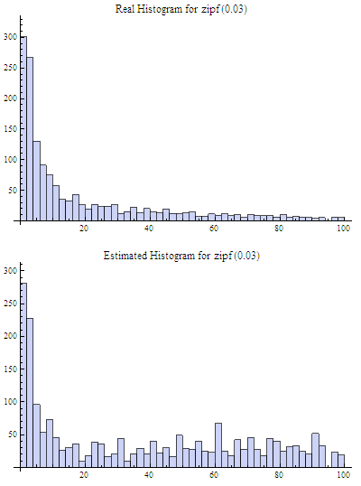
This enhancement can significantly improve accuracy of the Count-Min structure. For example, compare the histograms below with the first histograms for Count-Min sketch (both techniques used a sketch of size 3×64 and 8500 elements were added to it):

Count-Min sketches are applicable to the following problem: Find all elements in the data set with the frequencies greater than k percent of the total number of elements in the data set.（获取频率大于k%的元素总数，使用heap作为辅助） The algorithm is straightforward:（

• Maintain a standard Count-Min sketch during the scan of the data set and put all elements into it.
• Maintain a heap of top elements, initially empty, and a counter N of the total number of already process elements.
• For each element in the data set:
  • Put the element to the sketch
  • Estimate the frequency of the element using the sketch. If frequency is greater than a threshold (k*N), then put the element to the heap. Heap should be periodically or continuously cleaned up to remove elements that do not meet the threshold anymore.

这个过程应该是：1. 维护最小堆 2. 每次到达新元素的时候

• 估计这个元素出现的次数，如果 counter >= k * N的话，那么放入最小堆
• 调整最小堆：不断地pop元素，直到top元素 counter >= k * N.

如果这里的top-k里面的k不是percentage，而是具体数值的话，那么这个算法就更加简单。

In general, the top-k problem makes sense only for skewed data, so usage of Count-Min sketches is reasonable in this context.（因为使用的是count-min sketch算法因此只能针对skewed dataset使用）

这个算法还是比较好理解的。数据结构里面保留一定数目的槽位，添加value的时候增加其frequency counter. 如果达到槽位上限的话，那么就删除frequency counter最低的元素。

不过实现起来好像细节还蛮多的。我考虑实现办法可能是个双向链表，节点里面有两个字段：

1. values 所有落在这个节点的元素
2. count 这些元素出现的次数

假设新到达一个元素x的话

• 遍历整个链表，判断x是否在某个节点上
• 如果在这个节点上
  • 将x移到下一个节点，如果count匹配的话
  • 否则就新开辟一个节点
• 如果不在任何节点上，就删除头部节点创建新节点
• 保证长度上限是k

Basically, Stream-Summary traces a fixed number (a number of slots) of elements that presumably are most frequent ones. If one of these elements occurs in the stream, the corresponding counter is increased. If a new, non-traced element appears, it replaces the least frequent traced element and this kicked out element become non-traced.

The estimation procedure for most frequent elements and corresponding frequencies is quite obvious because of simple internal design of the Stream-Summary structure. Indeed, one just need to scan elements in the buckets that correspond to the highest frequencies. Nevertheless, Stream-Summary is able not only to provide estimates, but to answer are these estimates exact (guaranteed) or not. Computation of these guarantees is not trivial, corresponding algorithms are described in (8) （可以在上面做改进判断这个estimates是否准确，但是这个改进似乎并不直接）

In theory, one can process a range query (something like SELECT count(v) WHERE v >= c1 AND v < c2) using a Count-Min sketch enumerating all points within a range and summing estimates for corresponding frequencies. However, this approach is impractical because the number of points within a range can be very high and accuracy also tends to be inacceptable because of cumulative error of the sum.（对于范围查询可以枚举[c1,c2)所有的value，然后使用count-min sketch来得到count. 但是这个算法并不实际因为这个range可能非常大并且误差也很大，因为全部存放在一个sketch上面）

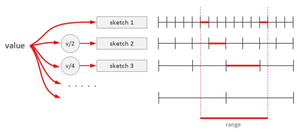
Nevertheless, it is possible to overcome these problems using multiple Count-Min sketches. The basic idea is to maintain a number of sketches with the different “resolution”, i.e. one sketch that counts frequencies for each value separately, one sketch that counts frequencies for pairs of values (to do this one can simply truncate a one bit of a value on the sketch’s input), one sketch with 4-items buckets and so on. The number of levels equals to logarithm of the maximum possible value. This schema is shown in the right part of the following picture:（可以使用都个count-min sketch来解决这个问题，这个也可以使用count-mean-min sketch来做）

这个地方非常巧妙。以第二个sketch为例，最后v和(v+1)会放到一个cell下面，而以第三个sketch为例，最后v,v+1,v+2,v+3会放到一个cell下面。然后再取的时候，假设range是[c1,c2]并且有5个sketch的话，从上而下我们分别称为1-sketch,2-sketch,4-sketch,8-sketch,16-sketch.那么最下面取的部分就是[(c1 + 15) / 16, c2 / 16]，排除这个部分之后剩余的部分在8-sketch取，有点类似二分法，整个查询是一个树状结构。

每个sketch维护的是一个前缀出现的次数。前缀越长，cardinality越大，collision也就越大，error rare也就越大。我们在查询范围的时候根据需要选择合适的前缀。比如我们希望统计[127, 172)的元素出现次数，首先列举区间边界的二进制表示

• 127 = 0b01111111
• 172 = 0b10101100

如果我们选取的前缀是 0b0111 的话，那么在这个sketch上面查询这么几个数值然后叠加：0b0111 0b1000 0b1001 0b1010. 当然这种方式会存在很大的偏差，如果想减少偏差的话可以取更长的前缀。另外可以取动态前缀比如 0b0111 0b10000 0b10001 0b10010 0b10011 0b101000 0b101011. 如果前缀是32的话，那么就相当于退化到一开始的方式了。

Any range query can be reduced to a number of queries to the sketches of different level, as it shown in right part of the picture above. This approach (called dyadic ranges) allows one to reduce the number of computations and increase accuracy. An obvious optimization of this schema is to replace sketches by exact counters at the lowest levels where a number of buckets is small.

MADlib (a data mining library for PostgreSQL and Greenplum) implements this algorithm to process range queries and calculate percentiles on large data sets.

Bloom Filter is probably the most famous and widely used probabilistic data structure. There are multiple descriptions of the Bloom filter in the web, I provide a short overview here just for sake of completeness. Bloom filter is similar to Linear Counting, but it is designed to maintain an identity of each item rather than statistics. Similarly to Linear Counter, the Bloom filter maintains a bitset, but each value is mapped not to one, but to some fixed number of bits by using several independent hash functions. If the filter has a relatively large size in comparison with the number of distinct elements, each element has a relatively unique signature and it is possible to check a particular value – is it already registered in the bit set or not. If all the bits of the corresponding signature are ones then the answer is yes (with a certain probability, of course).

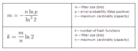
The following table contains formulas that allow one to calculate parameters of the Bloom filter as functions of error probability and capacity:

Bloom filter is widely used as a preliminary probabilistic test that allows one to reduce a number of exact checks. The following case study shows how the Bloom filter can be applied to the cardinality estimation.