Resilient Distributed Datasets: A Fault-Tolerant Abstraction for In-Memory Cluster Computing
Table of Contents
https://www.usenix.org/system/files/conference/nsdi12/nsdi12-final138.pdf @ 2012
1. Abstract
主要针对两类计算:迭代计算和交互分析,而这些都是针对批处理设计出来的系统的软肋。
- We present Resilient Distributed Datasets (RDDs), a distributed memory abstraction that lets programmers perform in-memory computations on large clusters in a fault-tolerant manner.
- RDDs are motivated by two types of applications that current computing frameworks handle inefficiently: iterative algorithms and interactive data mining tools.
- In both cases, keeping data in memory can improve performance by an order of magnitude. To achieve fault tolerance efficiently, RDDs provide a restricted form of shared memory, based on coarse-grained transformations rather than fine-grained updates to shared state. (关注于粗粒度的transformation,这点有点函数式编程和过程式编程的差异)
- However, we show that RDDs are expressive enough to capture a wide class of computations, including recent specialized programming models for iterative jobs, such as Pregel, and new applications that these models do not capture.
2. Introduction
当前分布式计算几个比较大的问题:
- Although current frameworks provide numerous abstractions for accessing a cluster’s computational resources, they lack abstractions for leveraging distributed memory. This makes them inefficient for an important class of emerging applications: those that reuse intermediate results across multiple computations.(缺少有效使用分布式内存的抽象)
- Data reuse is common in many iterative machine learning and graph algorithms, including PageRank, K-means clustering, and logistic regression. Another compelling use case is interactive data mining, where a user runs multiple adhoc queries on the same subset of the data.(没有办法重复地使用数据)
- Unfortunately, in most current frameworks, the only way to reuse data between computations (e.g., between two MapReduce jobs) is to write it to an external stable storage system, e.g., a distributed file system. This incurs substantial overheads due to data replication, disk I/O, and serializa-tion, which can dominate application execution times.(而现在对于数据的重用都是依赖于外部持久化系统比如分布式文件系统,data replication, disk I/O, 序列化都带来比较大的overhead)
- Recognizing this problem, researchers have developed specialized frameworks for some applications that require data reuse. For example, Pregel is a system for iterative graph computations that keeps intermediate data in memory, while HaLoop offers an iterative MapReduce interface. However, these frameworks only support specific computation patterns (e.g., looping a series of MapReduce steps), and perform data sharing implicitly for these patterns. They do not provide abstractions for more general reuse, e.g., to let a user load several datasets into memory and run ad-hoc queries across them.(针对特定场景设计系统,而没有通用的方案)
In this paper, we propose a new abstraction called resilient distributed datasets (RDDs) that enables efficient data reuse in a broad range of applications. RDDs are
- fault-tolerant,
- parallel data structures that let users explicitly persist intermediate results in memory,
- control their partitioning to optimize data placement,
- and ma-nipulate them using a rich set of operators.
The main challenge in designing RDDs is defining a programming interface that can provide fault tolerance efficiently.
- Existing abstractions for in-memory storage on clusters, such as distributed shared memory, keyvalue stores, databases, and Piccolo, offer an interface based on fine-grained updates to mutable state (e.g., cells in a table). With this interface, the only ways to provide fault tolerance are to replicate the data across machines or to log updates across machines. Both approaches are expensive for data-intensive workloads, as they require copying large amounts of data over the cluster network, whose bandwidth is far lower than that of RAM, and they incur substantial storage overhead.(允许细粒度地来更新状态,所以应对failover的实现办法只能够是replication)
- In contrast to these systems, RDDs provide an interface based on coarse-grained transformations (e.g., map, filter and join) that apply the same operation to many data items. This allows them to efficiently provide fault tolerance by logging the transformations used to build a dataset (its lineage) rather than the actual data. If a partition of an RDD is lost, the RDD has enough information about how it was derived from other RDDs to recompute just that partition. Thus, lost data can be recovered, often quite quickly, without requiring costly replication.(而RDD只允许粗粒度地更新状态,所以可以通过重算来处理failover)
- Although an interface based on coarse-grained transformations may at first seem limited, RDDs are a good fit for many parallel applications, because these applications naturally apply the same operation to multiple data items. Indeed, we show that RDDs can efficiently express many cluster programming models that have so far been proposed as separate systems.
3. Resilient Distributed Datasets (RDDs)
3.1. RDD Abstraction
- Formally, an RDD is a read-only, partitioned collection of records. RDDs can only be created through deterministic operations on either (1) data in stable storage or (2) other RDDs. We call these operations transformations to differentiate them from other operations on RDDs. Examples of transformations include map, filter, and join. (输入可以是持久介质以及其他RDD,包括一些变化操作)
- RDDs do not need to be materialized at all times. Instead, an RDD has enough information about how it was derived from other datasets (its lineage) to compute its partitions from data in stable storage. This is a powerful property: in essence, a program cannot reference an RDD that it cannot reconstruct after a failure.
- Finally, users can control two other aspects of RDDs: persistence and partitioning. Users can indicate which RDDs they will reuse and choose a storage strategy for them (e.g., in-memory storage). They can also ask that an RDD’s elements be partitioned across machines based on a key in each record. This is useful for placement optimizations, such as ensuring that two datasets that will be joined together are hash-partitioned in the same way.(用户可以控制持久化以及分片策略,改变分片策略对做join会很有帮助,可以做到co-partitioned join)
3.2. Spark Programming Interface
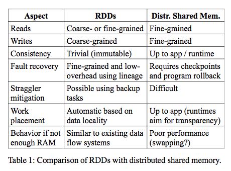
3.3. Advantages of the RDD Model
- The main difference between RDDs and DSM is that RDDs can only be created (“written”) through coarsegrained transformations, while DSM allows reads and writes to each memory location. This restricts RDDs to applications that perform bulk writes, but allows for more efficient fault tolerance. In particular, RDDs do not need to incur the overhead of checkpointing, as they can be recovered using lineage. Furthermore, only the lost partitions of an RDD need to be recomputed upon failure, and they can be recomputed in parallel on different nodes, without having to roll back the whole program.(不用去做checkpoint就可以做到fault-tolerant)
- A second benefit of RDDs is that their immutable nature lets a system mitigate slow nodes (stragglers) by running backup copies of slow tasks as in MapReduce. Backup tasks would be hard to implement with DSM, as the two copies of a task would access the same memory locations and interfere with each other’s updates. (可以很容易地复制计算单元,来处理出现straggler的情况)
- Finally, RDDs provide two other benefits over DSM. First, in bulk operations on RDDs, a runtime can schedule tasks based on data locality to improve performance. Second, RDDs degrade gracefully when there is not enough memory to store them, as long as they are only being used in scan-based operations. Partitions that do not fit in RAM can be stored on disk and will provide similar performance to current data-parallel systems.
3.4. Applications Not Suitable for RDDs
因为RDD是粗粒度的fault-tolerant,所以就不太适合需要精细控制fault-tolerant的场景,比如OLTP以及存储系统等。
As discussed in the Introduction, RDDs are best suited for batch applications that apply the same operation to all elements of a dataset. In these cases, RDDs can efficiently remember each transformation as one step in a lineage graph and can recover lost partitions without having to log large amounts of data. RDDs would be less suitable for applications that make asynchronous finegrained updates to shared state, such as a storage system for a web application or an incremental web crawler. For these applications, it is more efficient to use systems that perform traditional update logging and data checkpointing, such as databases, RAMCloud [25], Percolator [26] and Piccolo [27]. Our goal is to provide an efficient programming model for batch analytics and leave these asynchronous applications to specialized systems.
4. Spark Programming Interface
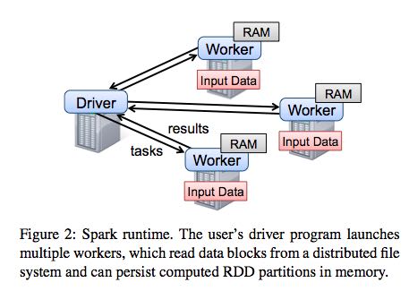
To use Spark, developers write a driver program that connects to a cluster of workers, as shown in Figure 2. The driver defines one or more RDDs and invokes ac- tions on them. Spark code on the driver also tracks the RDDs’ lineage. The workers are long-lived processes that can store RDD partitions in RAM across operations.
4.1. RDD Operations in Spark
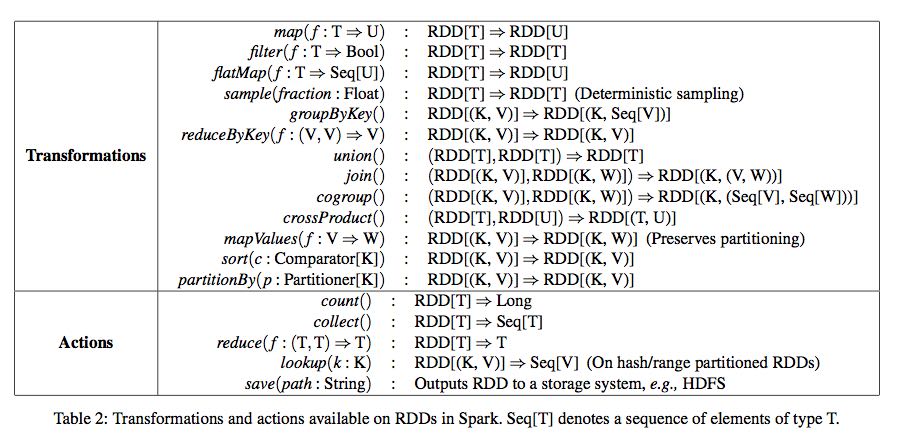
Table 2 lists the main RDD transformations and actions available in Spark. We give the signature of each oper- ation, showing type parameters in square brackets. Re- call that transformations are lazy operations that define a new RDD, while actions launch a computation to return a value to the program or write data to external storage.
5. Representing RDDs
One of the challenges in providing RDDs as an abstraction is choosing a representation for them that can track lineage across a wide range of transformations. Ideally, a system implementing RDDs should provide as rich a set of transformation operators as possible (e.g., the ones in Table 2), and let users compose them in arbitrary ways. We propose a simple graph-based representation for RDDs that facilitates these goals. We have used this representation in Spark to support a wide range of transformations without adding special logic to the scheduler for each one, which greatly simplified the system design.
In a nutshell, we propose representing each RDD through a common interface that exposes five pieces of information:
- a set of partitions, which are atomic pieces of the dataset;
- a set of dependencies on parent RDDs;
- a function for computing the dataset based on its parents;
- and metadata about its partitioning scheme
- and data placement.
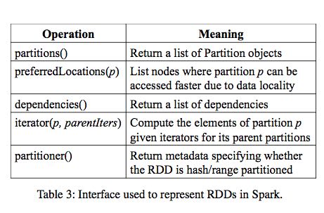
For example, an RDD representing an HDFS file has a partition for each block of the file and knows which machines each block is on. Meanwhile, the result of a map on this RDD has the same partitions, but applies the map function to the parent’s data when computing its elements.
我的理解是,RDD里面每个partition都要能够知道自己如何可以被计算出来。
操作按照是否需要shuffle分为了两类,并且按照这两类划分成为不同的stages.
The most interesting question in designing this interface is how to represent dependencies between RDDs. We found it both sufficient and useful to classify dependencies into two types:
- narrow dependencies(ND), where each partition of the parent RDD is used by at most one partition of the child RDD, (一个partition只会被child RDD中的一个partition所使用)
- wide dependencies(WD), where multiple child partitions may depend on it.(一个partition会被child RDD中的多个partition所使用)
For example, map leads to a narrow dependency, while join leads to to wide dependencies (unless the parents are hash-partitioned). Figure 4 shows other examples.
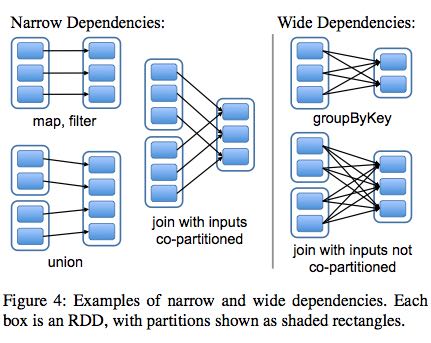
This distinction is useful for two reasons.
- First, narrow dependencies allow for pipelined execution on one cluster node, which can compute all the parent partitions. For example, one can apply a map followed by a filter on an element-by-element basis. In contrast, wide dependencies require data from all parent partitions to be available and to be shuffled across the nodes using a MapReducelike operation. (ND的结果RDD,每个partition在单个节点上面使用pipeline方式完成,各个partition的计算可以完全parallel. 而WD的结果RDD则需要parent RDD全部计算完成才能够计算)
- Second, recovery after a node failure is more efficient with a narrow dependency, as only the lost parent partitions need to be recomputed, and they can be recomputed in parallel on different nodes. In contrast, in a lineage graph with wide dependencies, a single failed node might cause the loss of some partition from all the ancestors of an RDD, requiring a complete re-execution.(ND比较容易recover只需要重新计算对应的parent RDD partition即可,而WD的recovery相对困难是因为需要从所有的parent RDD partition获取数据)
This common interface for RDDs made it possible to implement most transformations in Spark in less than 20 lines of code. Indeed, even new Spark users have implemented new transformations (e.g., sampling and various types of joins) without knowing the details of the scheduler. We sketch some RDD implementations below.
- HDFS files: The input RDDs in our samples have been files in HDFS. For these RDDs, partitions returns one partition for each block of the file (with the block’s offset stored in each Partition object), preferredLocations gives the nodes the block is on, and iterator reads the block.
- map: Calling map on any RDD returns a MappedRDD object. This object has the same partitions and preferred locations as its parent, but applies the function passed to map to the parent’s records in its iterator method.
- union: Calling union on two RDDs returns an RDD whose partitions are the union of those of the parents. Each child partition is computed through a narrow dependency on the corresponding parent.
- sample: Sampling is similar to mapping, except that the RDD stores a random number generator seed for each partition to deterministically sample parent records.
- join: Joining two RDDs may lead to either two narrow dependencies (if they are both hash/range partitioned with the same partitioner), two wide dependencies, or a mix (if one parent has a partitioner and one does not). In either case, the output RDD has a partitioner (either one inherited from the parents or a default hash partitioner).
这里我们使用spark-1.4.1运行一个例子, 来看看RDD中的这些概念. 首先我们用hdfs中读取一个文本文件上来, 指定分区数量为10.
scala> val rdd = sc.textFile("hdfs://192.168.3.3:8020/tmp/spark.org", 10)
15/09/11 16:53:21 INFO MemoryStore: ensureFreeSpace(231336) called with curMem=758866, maxMem=278302556
15/09/11 16:53:21 INFO MemoryStore: Block broadcast_12 stored as values in memory (estimated size 225.9 KB, free 264.5 MB)
15/09/11 16:53:21 INFO MemoryStore: ensureFreeSpace(19877) called with curMem=990202, maxMem=278302556
15/09/11 16:53:21 INFO MemoryStore: Block broadcast_12_piece0 stored as bytes in memory (estimated size 19.4 KB, free 264.4 MB)
15/09/11 16:53:21 INFO BlockManagerInfo: Added broadcast_12_piece0 in memory on 192.168.3.3:54538 (size: 19.4 KB, free: 265.3 MB)
15/09/11 16:53:21 INFO SparkContext: Created broadcast 12 from textFile at <console>:24
rdd: org.apache.spark.rdd.RDD[String] = MapPartitionsRDD[20] at textFile at <console>:24
然后我们可以查看这个rdd的partitions信息.
scala> rdd.partitions.size
15/09/11 16:53:42 INFO FileInputFormat: Total input paths to process : 1
res42: Int = 10

scala> rdd.partitions
res43: Array[org.apache.spark.Partition] = Array(org.apache.spark.rdd.HadoopPartition@99c,
 org.apache.spark.rdd.HadoopPartition@99d,
 org.apache.spark.rdd.HadoopPartition@99e,
 org.apache.spark.rdd.HadoopPartition@99f,
 org.apache.spark.rdd.HadoopPartition@9a0,
 org.apache.spark.rdd.HadoopPartition@9a1,
 org.apache.spark.rdd.HadoopPartition@9a2,
 org.apache.spark.rdd.HadoopPartition@9a3,
 org.apache.spark.rdd.HadoopPartition@9a4,
 org.apache.spark.rdd.HadoopPartition@9a5)

scala> rdd.partitions(0).index
res44: Int = 0
我们尝试找到这个rdd的HadoopRDD来看看它的preferredLocations. 可以看到这里Dependency是OneToOne, 也就是Narrow Dependency. paritioner为None, 表示使用默认分区函数
scala> rdd.dependencies
res45: Seq[org.apache.spark.Dependency[_]] = List(org.apache.spark.OneToOneDependency@4fec36f6)

scala> rdd.dependencies(0)
res46: org.apache.spark.Dependency[_] = org.apache.spark.OneToOneDependency@4fec36f6

scala> val hdfs = rdd.dependencies(0).rdd
hdfs: org.apache.spark.rdd.RDD[_] = hdfs://192.168.3.3:8020/tmp/spark.org HadoopRDD[19] at textFile at <console>:24

scala> hdfs.preferredLocations(hdfs.partitions(0))
res47: Seq[String] = ListBuffer()

scala> hdfs.partitioner
res48: Option[org.apache.spark.Partitioner] = None
6. Implementation
We have implemented Spark in about 14,000 lines of Scala. The system runs over the Mesos cluster manager, allowing it to share resources with Hadoop, MPI and other applications. Each Spark program runs as a separate Mesos application, with its own driver (master) and workers, and resource sharing between these applications is handled by Mesos. Spark can read data from any Hadoop input source (e.g., HDFS or HBase) using Hadoop’s existing input plugin APIs, and runs on an unmodified version of Scala.
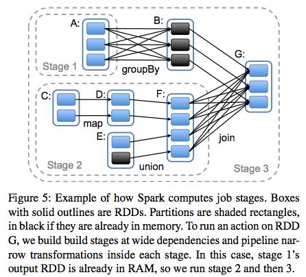
6.1. Job Scheduling
Overall, our scheduler is similar to Dryad’s, but it additionally takes into account which partitions of per-sistent RDDs are available in memory. Whenever a user runs an action (e.g., count or save) on an RDD, the scheduler examines that RDD’s lineage graph to build a DAG of stages to execute, as illustrated in Figure 5. Each stage contains as many pipelined transformations with narrow dependencies as possible. The boundaries of the stages are the shuffle operations required for wide dependencies, or any already computed partitions that can shortcircuit the computation of a parent RDD. The scheduler then launches tasks to compute missing partitions from each stage until it has computed the target RDD.(wild dependencies是每个stage的边界,stage内部都是narrow dependencies)
Our scheduler assigns tasks to machines based on data locality using delay scheduling. If a task needs to process a partition that is available in memory on a node, we send it to that node. Otherwise, if a task processes a partition for which the containing RDD provides pre- ferred locations (e.g., an HDFS file), we send it to those.(所谓的lazy scheduling是等待RDD确定位置之后,根据输入RDD partition的位置,将task移动到对应的位置上)
For wide dependencies (i.e., shuffle dependencies), we currently materialize intermediate records on the nodes holding parent partitions to simplify fault recovery, much like MapReduce materializes map outputs.If a task fails, we re-run it on another node as long as its stage’s parents are still available. If some stages have become unavailable (e.g., because an output from the “map side” of a shuffle was lost), we resubmit tasks to compute the missing partitions in parallel. We do not yet tolerate scheduler failures , though replicating the RDD lineage graph would be straightforward.(什么是scheduler failures? 现在在wide dependencies阶段都会对parent partitions进行物化,来节省recovery cost. 对于stage内部的话如果某个部分RDD存在的话,那么就会resuse, 否则触发重新计算的逻辑)
6.2. Interpreter Integration
Scala includes an interactive shell similar to those of Ruby and Python. Given the low latencies attained with in-memory data, we wanted to let users run Spark interactively from the interpreter to query big datasets.
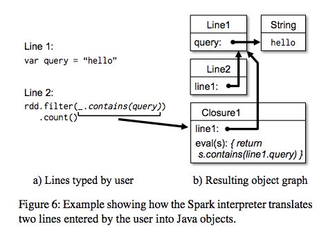
The Scala interpreter normally operates by compiling a class for each line typed by the user, loading it into the JVM, and invoking a function on it. This class includes a singleton object that contains the variables or functions on that line and runs the line’s code in an initialize method. For example, if the user types var x = 5 followed by println(x), the interpreter defines a class called Line1 containing x and causes the second line to compile to println(Line1.getInstance().x).(这是scala REPL实现原理?)
We made two changes to the interpreter in Spark:
- Class shipping: To let the worker nodes fetch the bytecode for the classes created on each line, we made the interpreter serve these classes over HTTP.(通过HTTP来实现class的分发)
- Modified code generation: Normally, the singleton object created for each line of code is accessed through a static method on its corresponding class. This means that when we serialize a closure referencing a variable defined on a previous line, such as Line1.x in the example above, Java will not trace through the object graph to ship the Line1 instance wrapping around x. Therefore, the worker nodes will not receive x. We modified the code generation logic to reference the instance of each line object directly.
Figure 6 shows how the interpreter translates a set of lines typed by the user to Java objects after our changes. (修改生成代码确保closure所引用的所有变量都会被包含)
6.3. Memory Management
Spark provides three options for storage of persistent RDDs:
- in-memory storage as deserialized Java objects, The first option provides the fastest performance, because the Java VM can access each RDD element natively.
- in-memory storage as serialized data, The second option lets users choose a more memory-efficient representation than Java object graphs when space is limited, at the cost of lower performance.
- and on-disk stor- age. The third option is useful for RDDs that are too large to keep in RAM but costly to recompute on each use.
To manage the limited memory available, we use an LRU eviction policy at the level of RDDs. When a new RDD partition is computed but there is not enough space to store it, we evict a partition from the least recently ac- cessed RDD, unless this is the same RDD as the one with the new partition. In that case, we keep the old partition in memory to prevent cycling partitions from the same RDD in and out. This is important because most oper- ations will run tasks over an entire RDD, so it is quite likely that the partition already in memory will be needed in the future. We found this default policy to work well in all our applications so far, but we also give users further control via a “persistence priority” for each RDD.(内存管理使用LRU淘汰策略。注意一个RDD partition不会触发相同RDD的其他partition被evicted,这点应该是比较实际的需求)
Finally, each instance of Spark on a cluster currently has its own separate memory space. In future work, we plan to investigate sharing RDDs across instances of Spark through a unified memory manager.
6.4. Support for Checkpointing
Although lineage can always be used to recover RDDs after a failure, such recovery may be time-consuming for RDDs with long lineage chains. Thus, it can be helpful to checkpoint some RDDs to stable storage.
In general, checkpointing is useful for RDDs with long lineage graphs containing wide dependencies. In contrast, for RDDs with narrow dependencies on data in stable storage, checkpointing may never be worthwhile. If a node fails, lost partitions from these RDDs can be recomputed in parallel on other nodes, at a fraction of the cost of replicating the whole RDD.(只是针对wide dependencies做checkpoint)
Spark currently provides an API for checkpointing (a REPLICATE flag to persist), but leaves the decision of which data to checkpoint to the user. However, we are also investigating how to perform automatic checkpointing. Because our scheduler knows the size of each dataset as well as the time it took to first compute it, it should be able to select an optimal set of RDDs to checkpoint to minimize system recovery time.(也提供API允许用户来做checkpoint. 也可以由系统进行启发式管理,比如存储相比重新计算成本更低的话,那么就值得做ckpt)
Finally, note that the read-only nature of RDDs makes them simpler to checkpoint than general shared memory. Because consistency is not a concern, RDDs can be written out in the background without requiring program pauses or distributed snapshot schemes.(因为RDD是完全只读的,所以RDD的checkpoint实现上比DSM的要简单不少,不需要像DSM一样需要做比较复杂的协调和控制时序)