Machine Learning by Andrew Ng
Table of Contents
- 1. definition
- 2. prerequisite
- 3. supervised learning
- 4. neural networks
- 5. support vector machine
- 6. advice for applying ML
- 7. advice for designing ML
- 8. unsupervised learning
- 9. dimensionality reduction
- 10. anomaly detection
- 11. recommender system
- 12. ML in large scale
- 13. appendix code
- 14. octave notes
https://class.coursera.org/ml-007
1. definition
T(task),E(experience),P(performance)
2. prerequisite
- linear algebra
- matrices / vectors # addition / subtraction/ multiplication / inversion / transposition
- some matrices are not invertible called singular / degenerate # redundant(linear dependent) or too many features
- pseudo inverse(pinv, works on matrix non-invertible) and inverse(inv)
- Octave #note: python-scikit-learn
3. supervised learning
- http://math.stackexchange.com/questions/141381/regression-vs-classification
- regression # continuous valued output.
- squared error function (as cost function) # ordinary-least-square 最小二乘法
- linear regression # 线性回归
- polynomial regression # 多项式回归
- classification # discrete valued output.
- decision boundary # 决策边界
- binary-class(negative/positive) vs. multi-class
- logistic regression # 逻辑回归
- sigmoid / logistic function
- g(x) = 1 / (1 + e^-x) [0, 1]
- interpretation of hypothesis output.
- p(y=0|x;theta) + p(y=1|x;theta) = 1 (for binary-class)
- h(x) = 1 / (1 + e^-(theta * x)) [0, 1]
- cost funciton = [-log(h(x)) if y = 1, -log(1-h(x)) if y = 0]
- => -(log(h(x)) * y + log(1-h(x)) * (1-y))
- SVM(support vector machine)
- training set / historical data set.
- input variables / features
- univariate # single input variable
- multivariate # multiple input variables.
- feature scaling / mean normalization
- output variables / targets
- feature scaling (otherwise more steps to find global minimum), approximately [-1,1]
- input variables / features
- hypothesis parameters(theta) and hypothesis(theta * x)
- cost function # 代价函数
- convex and non-convex function
- "batch" = uses all training set
- gradient descent algorithm # 梯度下降
- learning rate, derivative term.
- if learning rate is too small, converge rate could be low.
- if learning rate is too large, fail to converge or even diverge.
- gradient checking # 梯度检查
- optimization algorithm: conjugate gradient / BFGS / L-BFGS
- no need to manually peek learning rate
- faster than gradient descent
- provided cost function and partial derivatives
- 'fmincg' or 'fminunc' in Octave
- overfitting # 过拟合
- problem
- if underfit -> high bias
- if overfit -> high variance
- not generalize new examples
- generalization ability # 泛化能力
- addressing
- reduce number of features.
- manually select which features to keep
- model selection algorithm
- regularization # 正规化
- keep all features but reduce magnitude/values of parameters
- works well when we have a lot of features
- if regularization parameter is very large -> underfitting.
- L1 norm, L2 norm. L1范数和L2范数
- reduce number of features.
- problem
4. neural networks
- motivation # 神经网络
- complex non-linear classification / hypothesis # 针对复杂非线性分类
- many features -> too many polynomial terms.
- quantic x, then O(n^x).
- quadratic : O(n ^ 2)
- cubic: O(n ^ 3)
- background
- origins: algorithms that try to mimic the brain
- widely used in 80s and early 90s, popularity diminished in late 90s
- recent resurgence
- "one learning algorithm" hypothesis = cortex.
- model representation
- neuron in the brain # 神经元
- dendrite = input write # 树突
- axon = output write # 轴突
- cell body / nucleus # 核
- communicated by spike(pulse of electricity) # 电信号传输
- neuron model: logistic unit
- sigmoid (logistic) activation function # 激活函数
- hypothesis parameter = weight
- 数学之美C30: 神经元函数只能对输入变量线性组合后的结果进行一次非线性变换.
- layer: input/output/hidden
- a(i,j) = "activation" of unit i in layer j
- theta(j) = matrix of weights controlling function mapping from layer j to layer j+1
- if network has s(j) units in layer j, and s(j+1) units in layer j+1, then theta(j) is M(s(j+1), s(j)+1)
- forward propagation
- backward propagation
- neuron in the brain # 神经元
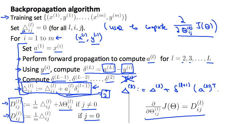
- backpropagation algorithm # 反向传播算法来计算参数导数
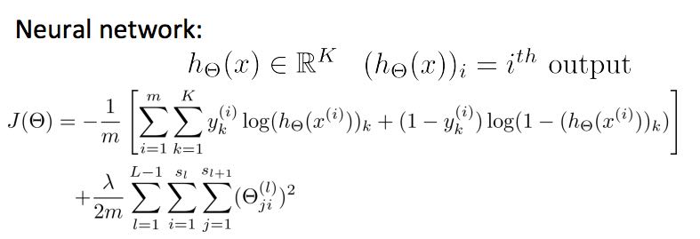
- general cost function
- delta(j,l) = "error" of node j in layer l
- intuition # use backpropagation algorithm to compute derivatives.
- implementation
- unroll parameters
- gradient checking(inefficient) to verify backprop derivatives
- initialize parameters randomly[symmetry breaking] (otherwise features are duplicated)
- putting together
- network architecture
- no. of input units: dimension of features
- no. of output units: number of classes
- hidden layer
- reasonable default: 1 hidden layer, or >1 hidden layer have same no. of hidden units in every layer(usually the more the better)
- no. of hidden units = [2,3,4] * no. input units.
- network size
- small # fewer parameters, more prone to underfitting, computationally cheaper.
- large # more parameters, more prone to overfitting, computationally more expensive.
- training a neural network
- randomly initialize weights
- for-loop to iterate each training samples.
- forward propagation to compute activation
- compute cost function
- backward propagation to compute partial derivatives
- gradient checking
- gradient descent algorithm
- network architecture
5. support vector machine
- alternative view of logistic regression
- SVM cost function # replace sigmoid function with two simple functions (cost0 and cost1)
- cost function = -y * cost1(tx) + (1-y) * cost0(tx)
- hypothesis: y = 1 if tx >=0. y = 0 otherwise.
- cost0和cost1实际上是合页损失函数(hinge loss function)
- SVM decision boundary / large margin intuition (if C very large) # SVM决策边界是找到完美划分的超平面
- kernel / kernel function # 核函数
- for more features
- to compute similarity (with landmarks) as more complex, non-linear features.
- gaussian kernel function.
- K(x,y,e) = exp ^ (-0.5 / e^2 * |x-y|^2)
- if e^2 is large, high bias and low variance
- if e^2 is small, low bias and high variance
- output range [0,1]
- how it works
- choose typical landmarks.
- compute similarity with landmarks as input [0,1]
- translate into a typical classifier problem.
- number of features == number of landmarks.
- practice
- liblinear, libsvm
- specify 1) choice of parameter C 2) kernel function
- no kernel / linear kernel function # n >> m
- gaussian kernel function # m >> n
- polynomial kernel function
- string kernel / chi-square kernel / histogram intersection kernel
6. advice for applying ML
- unacceptablely large errors in its predictions
- don't just use gut feelings and do the following things randomly
- get more training examples. (but not the more the better) => fix high variance
- try smaller sets of features. => fix high variance
- try getting additional features. => fix high bias
- try polynomial features. => fix high bias
- try decreasing/increasing lambda. => fix high bias/variance
- system diagnostics
- evaluating hypothesis
- split examples randomly into training set(70%) and test set(30%).
- see J_test(theta) is overfitting or not.
- model selection (for choosing polynomial terms and regularization)
- split examples randomly into training set(60%), cross validation set(20%), and test set(20%)
- use cross validation set to select model, and get estimate of generalization error.
- validation curves.
- high bias vs. variance
- bias > underfit: J_train(theta) is high, J_cv/test(theta) = J_train(theta)
- variance > overfit: J_train(theta) is low, but J_cv/test(theta) > J_train(theta)
- learning curves # J_cv/test(theta) and J_train(theta) over training set size
- if suffers from high bias, more training data will not help
- if suffers from high variance, more training data might help
- evaluating hypothesis
7. advice for designing ML
- numerical evaluation # a real number tells how well is your system. 使用一个数值来衡量系统
- error analysis # spot any systematic trend in what type of examples it is making errors on. 误差分析
- skewed classes.
- y = 1 in presence of rare class # 如果y_pred=0的话没有任何预测性但是accuracy准确率超高
- precision = true positive / [no. of predicted positive = (true pos + false pos)] # 精确度
- recall = true positive / [no. of actual positive = (true pos + false neg)] # 召回率
- good classifier: precision and recall are both high enough.
- but there are tradeoffs between both
- F1 score = 2 * P * R / (P + R)
- #note: see "anomaly detection select threshold" how to compute P,R, and F1.
- large data rationale
- assume features have sufficient information to predicate accurately
- useful test: give the input x, can a human expert confidently predict y?
8. unsupervised learning
- cluster algorithm
- cocktail party problem
- K-means algorithm
- cluster centroid
- K = cluster number, k = cluster index
- should have K < m
- choose K manually(most time) or with elbow method
- objective function = distances between training set and centroids.
- convex, but risk of local optima
- randomly choose centroids from training set.
- multiple random initialization
9. dimensionality reduction
- motivation # 维度降解
- data compression
- data visualization
- speed up learning algorithm
- PCA(principal component analysis) # 主成分分析
- find k vectors onto which to project the data
- minimize the projection error(different to linear regression)
- algorithm # reduce n dimensions to k dimensions
- sigma = 1/m * sum{X(i) * X(i)'}. X(i)~n*1, so sigma~n*n
- [U,S,V] = svd(sigma) # singular value decomposition
- U~n*n. use first k columns called U_reduce~(n*k)
- z = U_reduce' * X(i) ~ (k * n * n * 1) = (k*1)
- reconstruct: X_approx(i) = U_reduce * z ~ (n * k * k * 1) = (n*1)
- choose k # n% of variance is retained.
- n = sum{i=1,k}S_{ii} / sum{i=1,n}S_{ii} (S from svd, diagonal matrix)
- n = 99 typical value
- comments
- don't use PCA to prevent overfitting
- use raw data first, then consider PCA
10. anomaly detection
- gaussian distribution # 高斯分布
- X ~ N(u, e^2) # X distributed as N. where mean = u, variance = e^2
- p(x, u, e^2) = 1 / ((sqrt(2 * pi) * e)) * exp ^ { - (x-u)^2 / (2 * e^2) } # probability
- multivariate version # 多变量高斯分布
- to capture anomalous combination of values. computationally expensive.
- u~{n*1}, e~{n*n} (covariance matrix) # intuition. contour not axis aligned.
- p(x, u, e) = 1 / ((2 * pi) ^ (n/2) * sqrt(det(e))) * exp ^ {-0.5 * (x-u)' * e^-1 * (x-u)}
- u = 1/m * sum{x}, e = 1/m * sum{(x-u) * (x-u)'}
- #note: m > n, otherwise e is non-invertible.
- how it works # 我们假设特征数据符合高斯分布,所以异常数据点对应概率会非常低
- model p(x) from data
- p(x) < epsilon to decide if anomalous
- epsilon # p(x) is comparable for normal and anomalous examples.
- features to distinguish normal and anomalous examples.
- p(x) = p1(x1, u1, e1^2) * … pj(xj, uj, ej^2).. # j = # of features.
- if xj is not gaussian feature, transform it to fit into gaussian distribution. # 如果数据不满足高斯分布,那么要对数据做变换符合高斯分布
- vs. supervised learning
- anomaly detection
- # of positive cases is very small, while # of negative cases is very large
- many different types of "anomaly", hard to learn from positive cases what anomalies looks like
- future anomalies maybe very different to current ones.
- fraud detection, manufacturing, monitoring machines.
- supervised learning
- # of positive cases and negative cases are both very large
- enough positive cases to learn what positive cases look like
- future positive cases are similar to current ones.
- email spam, weather prediction, cancer classification.
- anomaly detection
11. recommender system
- content based recommendation
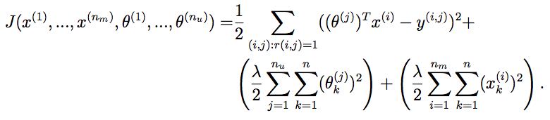
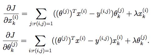
- collaborative filtering algorithm
- low rank matrix factorization
- random initialization to break symmetry
- content features to compute similarity between items
- mean normalization # 对于空值使用属性平均值代替
12. ML in large scale
- stochastic gradient descent algorithm # 随机梯度下降算法
- vs. batch gradient descent # 可以增量使用训练数据
- randomly shuffle dataset
- repeat for i = 1..m { for j = 0..n { update theta_j only use ith data } }
- move to global minimum generally, but not always in one iteration.
- convergence checking
- use averaged last k(say 1000) examples.
- the larger k, the smoother cost function curve.
- can slowly decrease learning rate over time for convergence.
- mini-batch gradient descent algorithm
- between batch and stochastic gradient descent
- use b(say 10) examples in one iteration
- take advantage of vectorization
- online learning
- map-reduce and data parallelism
- more data
- collect from multiple sources
- artificial data synthesis
- ceiling analysis
13. appendix code
13.1. feature normalization
function [X_norm, mu, sigma] = featureNormalize(X)
%FEATURENORMALIZE Normalizes the features in X
%   FEATURENORMALIZE(X) returns a normalized version of X where
%   the mean value of each feature is 0 and the standard deviation
%   is 1. This is often a good preprocessing step to do when
%   working with learning algorithms.

mu = mean(X);
X_norm = bsxfun(@minus, X, mu);

sigma = std(X_norm);
X_norm = bsxfun(@rdivide, X_norm, sigma);


% ============================================================

end
13.2. linear regression cost function
#note: works for polynomial regression too.
function [J, grad] = linearRegCostFunction(X, y, theta, lambda)
%LINEARREGCOSTFUNCTION Compute cost and gradient for regularized linear
%regression with multiple variables
%   [J, grad] = LINEARREGCOSTFUNCTION(X, y, theta, lambda) computes the
%   cost of using theta as the parameter for linear regression to fit the
%   data points in X and y. Returns the cost in J and the gradient in grad

% Initialize some useful values
m = length(y); % number of training examples

% You need to return the following variables correctly
J = 0;
grad = zeros(size(theta));

% ====================== YOUR CODE HERE ======================
% Instructions: Compute the cost and gradient of regularized linear
%               regression for a particular choice of theta.
%
%               You should set J to the cost and grad to the gradient.
%

diff = X * theta - y;
J = sum(diff .^ 2) * 0.5 / m;
t = theta;
t(1) = 0;
J += sum(t .^ 2) * lambda * 0.5 / m;
grad = ((X' * diff) + lambda * t) / m;

% =========================================================================

grad = grad(:);

end
13.3. neural network cost function
function [J grad] = nnCostFunction(nn_params, ...
                                   input_layer_size, ...
                                   hidden_layer_size, ...
                                   num_labels, ...
                                   X, y, lambda)
%NNCOSTFUNCTION Implements the neural network cost function for a two layer
%neural network which performs classification
%   [J grad] = NNCOSTFUNCTON(nn_params, hidden_layer_size, num_labels, ...
%   X, y, lambda) computes the cost and gradient of the neural network. The
%   parameters for the neural network are "unrolled" into the vector
%   nn_params and need to be converted back into the weight matrices.
%
%   The returned parameter grad should be a "unrolled" vector of the
%   partial derivatives of the neural network.
%

% Reshape nn_params back into the parameters Theta1 and Theta2, the weight matrices
% for our 2 layer neural network
Theta1 = reshape(nn_params(1:hidden_layer_size * (input_layer_size + 1)), ...
                 hidden_layer_size, (input_layer_size + 1));

Theta2 = reshape(nn_params((1 + (hidden_layer_size * (input_layer_size + 1))):end), ...
                 num_labels, (hidden_layer_size + 1));

% Setup some useful variables
m = size(X, 1);

% You need to return the following variables correctly
J = 0;
Theta1_grad = zeros(size(Theta1));
Theta2_grad = zeros(size(Theta2));

% ====================== YOUR CODE HERE ======================
% Instructions: You should complete the code by working through the
%               following parts.
%
% Part 1: Feedforward the neural network and return the cost in the
%         variable J. After implementing Part 1, you can verify that your
%         cost function computation is correct by verifying the cost
%         computed in ex4.m
%
% Part 2: Implement the backpropagation algorithm to compute the gradients
%         Theta1_grad and Theta2_grad. You should return the partial derivatives of
%         the cost function with respect to Theta1 and Theta2 in Theta1_grad and
%         Theta2_grad, respectively. After implementing Part 2, you can check
%         that your implementation is correct by running checkNNGradients
%
%         Note: The vector y passed into the function is a vector of labels
%               containing values from 1..K. You need to map this vector into a
%               binary vector of 1's and 0's to be used with the neural network
%               cost function.
%
%         Hint: We recommend implementing backpropagation using a for-loop
%               over the training examples if you are implementing it for the
%               first time.
%
% Part 3: Implement regularization with the cost function and gradients.
%
%         Hint: You can implement this around the code for
%               backpropagation. That is, you can compute the gradients for
%               the regularization separately and then add them to Theta1_grad
%               and Theta2_grad from Part 2.
%

X2 = [ones(m, 1)  X];
tx2 = X2 * Theta1';
hx2 = sigmoid(tx2);
X3 = [ones(m, 1) hx2];
tx3 = X3 * Theta2';
hx3 = sigmoid(tx3);
hy = zeros(m, num_labels);
for i = [1:m],
    hy(i, y(i)) = 1;
end;
J = sum(sum(log(hx3) .* (-hy) - log(1 - hx3) .* (1 - hy))) / m;

R = 0;
R += sum(sum(Theta1(:, 2:end) .^ 2));
R += sum(sum(Theta2(:, 2:end) .^ 2));
R *= lambda / m * 0.5;

J += R;

% -------------------------------------------------------------

d3 = hx3 - hy; # M * K
d2 = (d3 * Theta2)(:,2:end) .* sigmoidGradient(tx2); # M * H
Theta2_grad = d3' * X3 / m; # K * M * M * (H+1) = K * (H+1)
Theta1_grad = d2' * X2 / m; # H * M * M * (N+1) = H * (N+1)

t2 = Theta2;
t2(:,1) = 0;
t1 = Theta1;
t1(:,1) = 0;
Theta2_grad += t2 * lambda / m;
Theta1_grad += t1 * lambda / m;

% =========================================================================

% Unroll gradients
grad = [Theta1_grad(:) ; Theta2_grad(:)];


end
13.4. pca(principal compoenent analysis)
function [U, S] = pca(X)
%PCA Run principal component analysis on the dataset X
%   [U, S, X] = pca(X) computes eigenvectors of the covariance matrix of X
%   Returns the eigenvectors U, the eigenvalues (on diagonal) in S
%

% Useful values
[m, n] = size(X);

% You need to return the following variables correctly.
U = zeros(n);
S = zeros(n);

% ====================== YOUR CODE HERE ======================
% Instructions: You should first compute the covariance matrix. Then, you
%               should use the "svd" function to compute the eigenvectors
%               and eigenvalues of the covariance matrix.
%
% Note: When computing the covariance matrix, remember to divide by m (the
%       number of examples).
%

sigma = 1.0 / m * X' * X;
[U,S,_ ] = svd(sigma);


% =========================================================================

end
projectData
function Z = projectData(X, U, K)
%PROJECTDATA Computes the reduced data representation when projecting only
%on to the top k eigenvectors
%   Z = projectData(X, U, K) computes the projection of
%   the normalized inputs X into the reduced dimensional space spanned by
%   the first K columns of U. It returns the projected examples in Z.
%

% You need to return the following variables correctly.
Z = zeros(size(X, 1), K);

% ====================== YOUR CODE HERE ======================
% Instructions: Compute the projection of the data using only the top K
%               eigenvectors in U (first K columns).
%               For the i-th example X(i,:), the projection on to the k-th
%               eigenvector is given as follows:
%                    x = X(i, :)';
%                    projection_k = x' * U(:, k);
%

U_reduce = U(:, 1:K);

Z = X * U_reduce;


% =============================================================

end
recoverData
function X_rec = recoverData(Z, U, K)
%RECOVERDATA Recovers an approximation of the original data when using the
%projected data
%   X_rec = RECOVERDATA(Z, U, K) recovers an approximation the
%   original data that has been reduced to K dimensions. It returns the
%   approximate reconstruction in X_rec.
%

% You need to return the following variables correctly.
X_rec = zeros(size(Z, 1), size(U, 1));

% ====================== YOUR CODE HERE ======================
% Instructions: Compute the approximation of the data by projecting back
%               onto the original space using the top K eigenvectors in U.
%
%               For the i-th example Z(i,:), the (approximate)
%               recovered data for dimension j is given as follows:
%                    v = Z(i, :)';
%                    recovered_j = v' * U(j, 1:K)';
%
%               Notice that U(j, 1:K) is a row vector.
%

U_reduce = U(:, 1:K);

X_rec = Z * U_reduce';

% =============================================================

end
13.5. gaussian distribution
compute mean and variance of X
function [mu sigma2] = estimateGaussian(X)
%ESTIMATEGAUSSIAN This function estimates the parameters of a
%Gaussian distribution using the data in X
%   [mu sigma2] = estimateGaussian(X),
%   The input X is the dataset with each n-dimensional data point in one row
%   The output is an n-dimensional vector mu, the mean of the data set
%   and the variances sigma^2, an n x 1 vector
%

% Useful variables
[m, n] = size(X);

% You should return these values correctly
mu = zeros(n, 1);
sigma2 = zeros(n, 1);

% ====================== YOUR CODE HERE ======================
% Instructions: Compute the mean of the data and the variances
%               In particular, mu(i) should contain the mean of
%               the data for the i-th feature and sigma2(i)
%               should contain variance of the i-th feature.
%

mu = mean(X)';
# xu = X - mu';
# sigma2 = 1.0 / m * sum(xu .^ 2)';
sigma2 = (m-1) / m * var(X)';

% =============================================================


end
compute probability
function p = multivariateGaussian(X, mu, Sigma2)
%MULTIVARIATEGAUSSIAN Computes the probability density function of the
%multivariate gaussian distribution.
%    p = MULTIVARIATEGAUSSIAN(X, mu, Sigma2) Computes the probability
%    density function of the examples X under the multivariate gaussian
%    distribution with parameters mu and Sigma2. If Sigma2 is a matrix, it is
%    treated as the covariance matrix. If Sigma2 is a vector, it is treated
%    as the \sigma^2 values of the variances in each dimension (a diagonal
%    covariance matrix)
%

k = length(mu);

if (size(Sigma2, 2) == 1) || (size(Sigma2, 1) == 1)
    Sigma2 = diag(Sigma2);
end

X = bsxfun(@minus, X, mu(:)');
p = (2 * pi) ^ (- k / 2) * det(Sigma2) ^ (-0.5) * ...
    exp(-0.5 * sum(bsxfun(@times, X * pinv(Sigma2), X), 2));

end
13.6. anomaly detection select threshold
function [bestEpsilon bestF1] = selectThreshold(yval, pval)
%SELECTTHRESHOLD Find the best threshold (epsilon) to use for selecting
%outliers
%   [bestEpsilon bestF1] = SELECTTHRESHOLD(yval, pval) finds the best
%   threshold to use for selecting outliers based on the results from a
%   validation set (pval) and the ground truth (yval).
%

bestEpsilon = 0;
bestF1 = 0;
F1 = 0;

stepsize = (max(pval) - min(pval)) / 1000;
for epsilon = min(pval):stepsize:max(pval)

    % ====================== YOUR CODE HERE ======================
    % Instructions: Compute the F1 score of choosing epsilon as the
    %               threshold and place the value in F1. The code at the
    %               end of the loop will compare the F1 score for this
    %               choice of epsilon and set it to be the best epsilon if
    %               it is better than the current choice of epsilon.
    %
    % Note: You can use predictions = (pval < epsilon) to get a binary vector
    %       of 0's and 1's of the outlier predictions

    cv_pred = pval < epsilon;
    tp = sum((cv_pred == 1) & (yval == 1));
    fp = sum((cv_pred == 1) & (yval == 0));
    fn = sum((cv_pred == 0) & (yval == 1));
    prec = tp / (tp + fp);
    recall = tp / (tp + fn);
    F1 = 2 * prec * recall / (prec + recall);

    % =============================================================

    if F1 > bestF1
       bestF1 = F1;
       bestEpsilon = epsilon;
    end
end

end
13.7. collaborative filtering cost function
function [J, grad] = cofiCostFunc(params, Y, R, num_users, num_movies, ...
                                  num_features, lambda)
%COFICOSTFUNC Collaborative filtering cost function
%   [J, grad] = COFICOSTFUNC(params, Y, R, num_users, num_movies, ...
%   num_features, lambda) returns the cost and gradient for the
%   collaborative filtering problem.
%

% Unfold the U and W matrices from params
X = reshape(params(1:num_movies*num_features), num_movies, num_features);
Theta = reshape(params(num_movies*num_features+1:end), ...
                num_users, num_features);


% You need to return the following values correctly
J = 0;
X_grad = zeros(size(X));
Theta_grad = zeros(size(Theta));

% ====================== YOUR CODE HERE ======================
% Instructions: Compute the cost function and gradient for collaborative
%               filtering. Concretely, you should first implement the cost
%               function (without regularization) and make sure it is
%               matches our costs. After that, you should implement the
%               gradient and use the checkCostFunction routine to check
%               that the gradient is correct. Finally, you should implement
%               regularization.
%
% Notes: X - num_movies  x num_features matrix of movie features
%        Theta - num_users  x num_features matrix of user features
%        Y - num_movies x num_users matrix of user ratings of movies
%        R - num_movies x num_users matrix, where R(i, j) = 1 if the
%            i-th movie was rated by the j-th user
%
% You should set the following variables correctly:
%
%        X_grad - num_movies x num_features matrix, containing the
%                 partial derivatives w.r.t. to each element of X
%        Theta_grad - num_users x num_features matrix, containing the
%                     partial derivatives w.r.t. to each element of Theta
%

xt = X * Theta'; % m * n * n * u = m * u
df = (xt- Y) .* R; % m * u
J = 0.5 * sum(sum(df .^ 2));
J += 0.5 * lambda * (sum(sum(Theta .^ 2)) + sum(sum(X .^ 2)));


X_grad = df * Theta; % m * u * u * n = m * n;
X_grad += lambda * X;

Theta_grad = df' * X; % u * m * m * n = u * n;
Theta_grad += lambda * Theta;

% =============================================================

grad = [X_grad(:); Theta_grad(:)];

end
14. octave notes
- basic syntax
- ==(equal), ~=(not equal), xor(a,b), PS1('new promot: ') starts comment with %
- ; to supersede output
- m(:) expand m to a single column vector.
- m(i,j) could be used as left operand. And for i,j could be
- [a b] which means ath and bth elements.
- or s:i:e/s:e which is shorthand of [a,b] # end as a keyword.
- or : which means every elements.
- output control
- disp(value) to print value
- sprintf to format string in C syntax.
- format long/short # change output format of numerical values.
- hist(matrix, [bucket]) to plot histogram of matrix.
- generate matrix
- [a b ; c d; e f ]. 3 * 2 matrix.
- [start : interval : end] / [ start : end ] as interval = 1.
- ones/zeros(m,n) m * n matrix with elements are all 0/1.
- rand(m,n) m * n matrix with uniform distributed random elements in range [0,1]
- randn Gaussian distribution with mean = 0 and standard deviation = 1
- eye(n) n * n identity matrix
- import/export data
- size, who/whos, clear [<value>],
- load <file>, save <file> <value> [-ascii % readable form]
- compute command
- . means elements wise operation.
- A .* B , A .^ 2 , 1 ./ A , A .+ 1 , A .- 1
- log, exp, abs, -(neg), <
- A * B
- A' # tranpose
- max/find/magic/sum/prod/floor/ceil/flipud/pivn
- drawing command
- plot(x,y)
- hold on # plot new figure on old one.
- xlabel / ylabel / legend / title / print # output to file / close / axis
- figure # create figure / clf # clear figure
- subplot(m,n,ind) # divides plot a m*n grid, and access ind th
- "imagesc(<matrix>) , colorbar , colormap gray;"
- flow control
- for i=<range>[1:10], <stmt> end;
- if <cond>, <stmt> end; / elseif / else
- while <cond>, <stmt> end;
- break/continue
- function definition resides in function_name.m
- function y = <name>(x)
- function [y1,y2] = <name>(x)
- y = x * 2
- name(x) to call function.
- addpath to add path in order to find function file.