Data Structures and Algorithms for Big Databases
Table of Contents
1. Overview
- Michael A. Bender @ Stony Brook & Tokutek
- Bradley C. Kuszmaul @ MIT & Tokutek
Funny tradeoff in ingestion, querying, freshness
- “I'm trying to create indexes on a table with 308 million rows. It took ~20 minutes to load the table but 10 days to build indexes on it.”
- “Select queries were slow until I added an index onto the timestamp field…Adding the index really helped our reporting, BUT now the inserts are taking forever.”
- “They indexed their tables, and indexed them well, And lo, did the queries run quick! But that wasn’t the last of their troubles, to tell-Their insertions, like treacle, ran thick.”
- 在DBMS设计上如何使得insert,query,index高效快速
What we mean by Big Data
- We don’t define Big Data in terms of TB, PB, EB. 不以数据量来定义大数据
- By Big Data, we mean
- The data is too big to fit in main memory. 数据不能够全部放在内存中
- We need data structures on the data. 设计良好的数据结构存储数据
- Words like “index” or “metadata” suggest that there are underlying data structures
- These data structures are also too big to fit in main memory.
Topics and Outline for this Tutorial
- I/O model and cache-oblivious analysis. IO模型和cache-oblivious分析
- Write-optimized data structures. 写优化数据结构
- How write-optimized data structures can help file systems. 写优化数据结构如何影响文件系统
- Block-replacement algorithms. block替换算法/Cache替换算法
- Indexing strategies. 索引策略
- Log-structured merge trees. LSM
- Bloom filters.
2. I/O Model and Cache-Oblivious
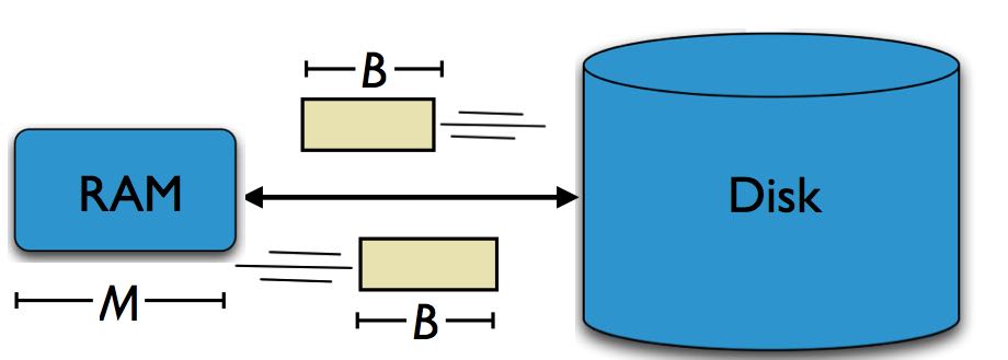
2.1. Modeling I/O Using the Disk Access Model
- How computation works:
- Data is transferred in blocks between RAM and disk. 考虑数据在RAM和disk之间传输
- The # of block transfers dominates the running time. 传输的block数目决定了运行时间
- Goal: Minimize # of block transfers
- Performance bounds are parameterized by block size B, memory size M, data size N.
merge-sort analysis非常精辟,每次merge run是M/B. 这点非常重要,因此我们每次读取disk都是整个block读取的,因此最多hold M/B ways. 这样可以看出,每次merge的fanout是M/B. 总共需要处理N/B block,因此tree depth是在log(M/b)(N/B). 而每个depth操作代价是N/B.
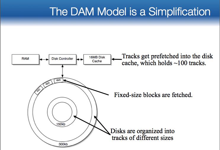
- The DAM Model is a Simplification
- ignores CPU costs and 没有考虑到CPU开销,仅仅是考虑IO开销
- assumes that all block accesses have the same cost. 假设所有的block访问时间都是相同的
2.2. Cache-Oblivious Analysis
- Cache-oblivious analysis:
- Parameters B, M are unknown to the algorithm or coder.
- Performance bounds are parameterized by block size B, memory size M, data size N.
- Goal (as before): Minimize # of block transfer
- Cache-oblivious algorithms work for all B and M
- It’s better to optimize approximately for all B, M than to pick the best B and M.
- #note: 所谓的cache-oblivious就是忘记B,M这些参数,算法的优化不要依赖B,M这些参数的组合,而必须使得所有任意的B,M组合都足够好
3. Write-Optimized Data Structures
- Data structures: [O'Neil,Cheng, Gawlick, O'Neil 96], [Buchsbaum, Goldwasser, Venkatasubramanian, Westbrook 00], [Argel 03], [Graefe 03], [Brodal, Fagerberg 03], [Bender, Farach,Fineman,Fogel, Kuszmaul, Nelson’07], [Brodal, Demaine, Fineman, Iacono, Langerman, Munro 10], [Spillane, Shetty, Zadok, Archak, Dixit 11].
- Systems: BigTable, Cassandra, H-Base, LevelDB, TokuDB.
- #note: 大部分都是LSM实现
理论上最优化的query/insert/delete之间的逻辑复杂度如下:
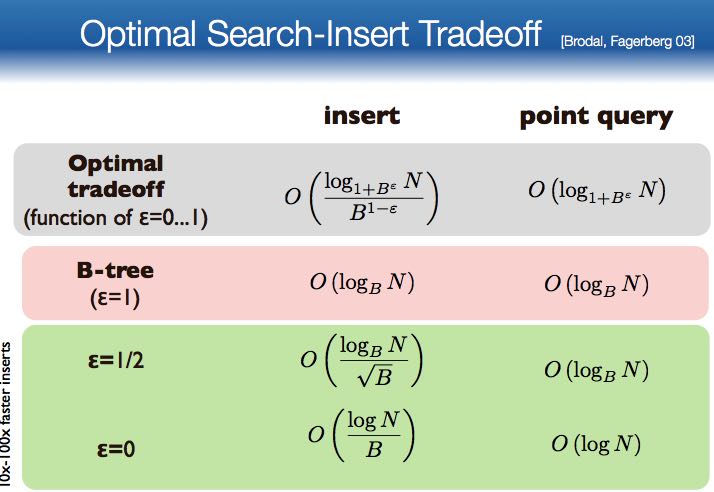
或许上面这个图不是很好理解,但是在性能上曲线如下: 可以看到查询最快的是btree, insert最快的是logging
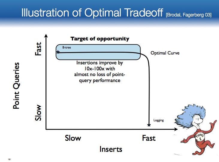
我们所要做的就是在曲线变化的中间找到最优的写性能
事实上非常有意思的事情是, The right read-optimization is write-optimization
- The right index makes queries run fast. 正确的索引可以使得查询非常快速
- Write-optimized structures maintain indexes efficiently. 而写优化数据结构可以有效地维护索引
- Fast writing is a currency we use to accelerate queries. Better indexing means faster queries.
- Write-optimized structures can significantly mitigate the insert/query/freshness tradeoff. 写优化的数据结构可以在insert/query/freshness上达到平衡
Optimal read-write tradeoff: Easy Full featured: Hard 实现需要考虑如下问题:
- Variable-sized rows
- Concurrency-control mechanisms
- Multithreading
- Transactions, logging, ACID-compliant crash recovery
- Optimizations for the special cases of sequential inserts and bulk loads
- Compression
- Backup
4. TokuFS–How to Make a Write-Optimized File System
- Microdata is the Problem 重点解决元数据存储问题
5. Paging
- Paging Algorithms
- LRU (least recently used) Discard block whose most recent access is earliest.
- FIFO (first in, first out) Discard the block brought in longest ago.
- LFU (least frequently used) Discard the least popular block.
- Random Discard a random block.
- LFD (longest forward distance)=OPT [Belady 69] Discard block whose next access is farthest in the future. optimal
6. What to Index
- Indexes provide query performance
- Indexes can reduce the amount of retrieved data.
- Less bandwidth, less processing, …
- Indexes can improve locality.
- Not all data access cost is the same
- Sequential access is MUCH faster than random access
- Indexes can presort data.
- GROUP BY and ORDER BY queries do post-retrieval work
- Indexing can help get rid of this work
7. Log Structured Merge Trees
#todo: LSM algorithm analysis
- Log structured merge trees are write-optimized data structures developed in the 90s.
- Over the past 5 years, LSM trees have become popular (for good reason).
- Accumulo, Bigtable, bLSM, Cassandra, HBase, Hypertable, LevelDB are LSM trees (or borrow ideas).
- http://nosql-database.org lists 122 NoSQL databases. Many of them are LSM trees.
- Looking in all those trees is expensive, but can be improved by
- caching,
- Bloom filters, and
- fractional cascading. 根据在上一个subtree query结果帮助在下一个subtree query.
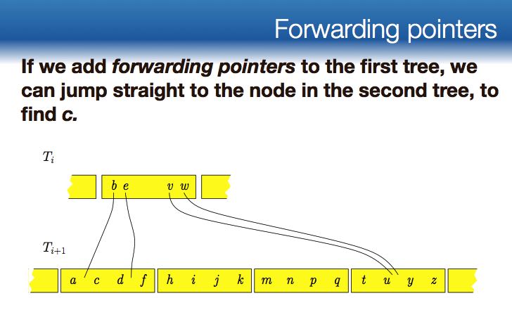
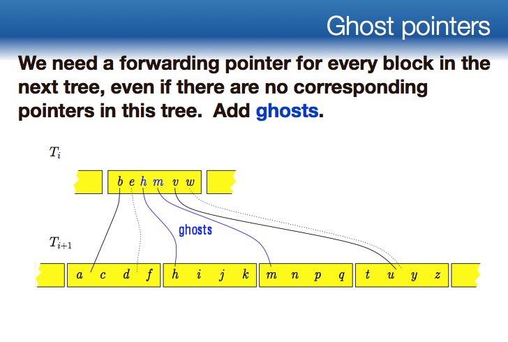
- Instead of avoiding searches in trees, we can use a technique called fractional cascading to reduce the cost of searching each B-tree to O(1).
- Idea: We’re looking for a key, and we already know where it should have been in T3, try to use that information to search T4.
- forward pointer and ghost pointer
8. Bloom Filters
- If n items are in an array of size m, then the chances of getting a YES answer on an element that is not there is 1 - e^(-n /m)
- Counting bloom filters [Fan, Cao, Almeida, Broder 2000] allow deletions by maintaining a 4-bit counter instead of a single bit per object.
- Buffered Bloom Filters [Canin, Mihaila, Bhattacharhee, and Ross, 2010] employ hash localization to direct all the hashes of a single insertion to the same block.
- Cascade Filters [Bender, Farach-Colton, Johnson, Kraner, Kuszmaul, Medjedovic, Montes, Shetty, Spillane, Zadok 2011] support deletions, exhibit locality for queries, insert quickly, and are cache-oblivious.
9. Closing Words
- Big Data Epigrams
- The problem with big data is microdata.
- Sometimes the right read optimization is a write-optimization.
- As data becomes bigger, the asymptotics become more important.
- Life is too short for half-dry white-board markers and bad sushi.